11 · N² is the enemy

Acts I–III were about getting the answer right. Act IV is about getting it fast enough to matter, because correctness you can’t afford isn’t much use. And the thing standing in the way has been sitting in plain sight since chapter 2: the moment matrix is dense, and dense matrices scale viciously.

The wall

Every one of the N basis functions interacts with every other, so Z is a full N × N matrix. That costs on three axes at once. Filling it touches every pair — O(N²) kernel evaluations. Factoring it to solve Z·I = V is Gaussian elimination — O(N³). Storing it is O(N²) complex numbers. Push N up and watch:

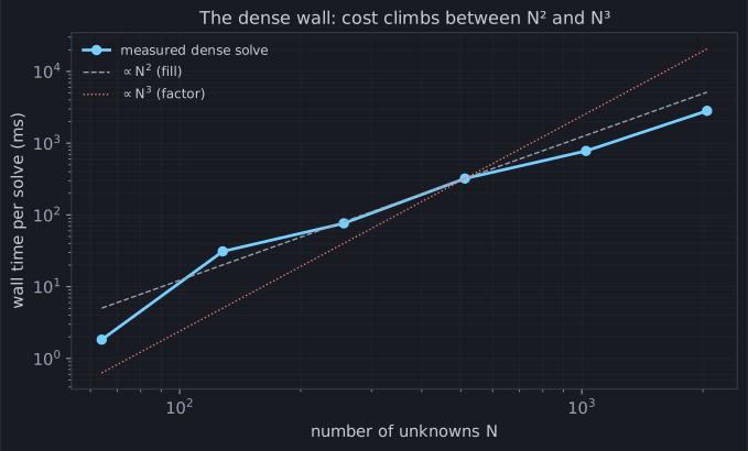
For the specimen dipole, N = 21 and none of this matters — the whole solve is a millisecond. But N is set by size in wavelengths, and it climbs fast: a big wire array, a log-periodic with dozens of elements, a structure many wavelengths across, and N is in the thousands. At N = 2048 a single solve is already seconds and the matrix is tens of megabytes; a few doublings past that and you’re out of memory before you’re out of patience. The O(N³) factor is the part that eventually wins, and it wins ugly.

Sweeps: the same wall, M times

It gets worse, because you rarely want one frequency. A ham wants the impedance across a band — the chapter 3 sweep. Done naively, an M-point sweep is M full solves: fill and factor, from scratch, M times.

Except most of that work doesn’t depend on frequency. Remember chapter 6’s static moments — the singular integrals were called static precisely because they don’t move with k. The geometry doesn’t change across a sweep either. So momwire’s swept solver (compute_impedance_swept) computes the frequency-independent parts once and reuses them at every point:

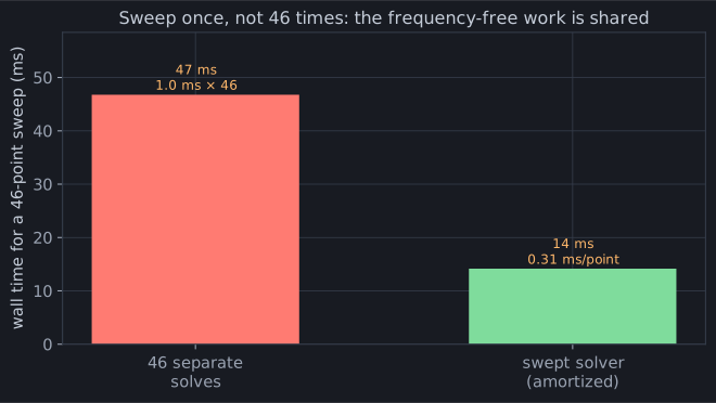
Forty-six frequencies for well under the price of forty-six solves — each extra point is a fraction of a cold one. And because building all those per-k matrices at once could blow up memory, the swept path fills them in batches under a budget (swept_mem_mb, default 256 MB, via _swept_batched_z_chunks) — you get the amortization without the memory spike.

But the wall is still there

Amortizing a sweep is a discount on the constant, not a change in the exponent. A single solve of a genuinely large structure is still O(N³), and no amount of sweep-sharing rescues it. To actually break the wall you have to attack the N² itself — to stop treating the matrix as N² independent numbers.

And here’s the opening, and it’s been visible since chapter 2. Go back and look at that moment-matrix heatmap: a screaming diagonal, and then vast, smooth, boring regions off it, where the field of one distant chunk of wire barely varies across another. All those far-apart interactions carry almost no independent information. The matrix is dense, but it is not full of content — it is, in a precise sense, secretly small. Chapter 12 makes that precise and cashes it in.