9 · Real dirt, cheap

Chapter 8’s mirror was perfect: |Γ| = 1, every watt bounced straight back. Actual ground is nothing like that. It’s a lossy dielectric — average soil has a relative permittivity around 13 and a conductivity around 0.005 S/m — and when a wave hits it, some reflects, some refracts down and is absorbed, and the part that does reflect comes back weaker and phase-shifted. The image is still there; it’s just dim, and how dim depends on the angle.

A reflection coefficient instead of a perfect image

The physics of “how much reflects off a flat interface” is two centuries old: Fresnel’s reflection coefficient Γ. For the ground it’s complex — the soil’s loss enters as a complex permittivity ε̃ = εr − jσ/ωε₀ — and it depends on both the grazing angle and the polarization:

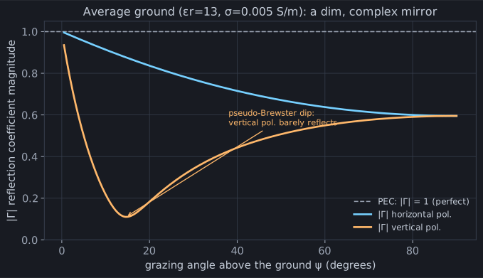
Nothing about this is 1. Horizontally polarized waves reflect fairly well at low angles and fade toward 0.6 overhead. Vertically polarized waves do something dramatic — near the pseudo-Brewster angle (~15° here) the ground barely reflects them at all, |Γ| diving toward 0.1. That single dip is why vertical antennas over real ground behave so differently from the textbook-perfect case.

And here’s the bargain: putting this into the solver costs almost nothing beyond chapter 8. It’s the same image, with its contribution multiplied by Γ before it’s added to each matrix entry — one complex, angle-dependent weight per interaction, no new unknowns (_ground_refl.py; NEC calls this ground mode “GN 0”). In momwire it’s one more argument, ground_eps=(13, 0.005).

Good until it isn’t

So how good is a weighted mirror? Put it up against the exact answer — the full Sommerfeld solve of chapter 10 — across height:

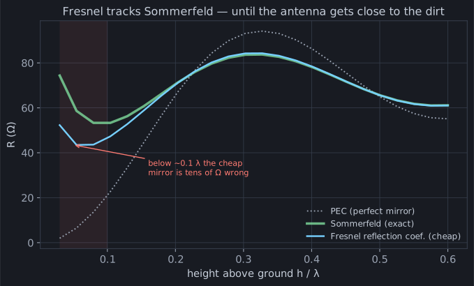
Two things to take away. First, the good news: from about 0.15 λ upward the cheap model is indistinguishable from the exact one — a fraction of an ohm apart, for a fraction of the cost. For the vast majority of real antennas, a half-wave or more off the ground, the Fresnel reflection coefficient simply is the right answer.

Second, the honest news: below about 0.1 λ it falls apart, tens of ohms adrift. The reflection-coefficient picture assumes the antenna’s field arrives at the ground as a plane wave reflecting at a definite angle. When the wire is a stone’s throw from the dirt, that assumption fails — the near field is not a plane wave, and no single Γ(angle) can describe it. Notice, though, that even where it’s wrong, it’s wrong in the right direction: unlike the PEC image, which shorts a low horizontal dipole to nearly zero, real lossy ground keeps R up in the 60–75 Ω range — a low dipole over dirt still radiates. Fresnel gets that qualitative rescue, just not the exact number.

Run it yourself

import numpy as np
from momwire import BSplineSolver

# horizontal dipole, 0.2 lambda up, over average ground
wire = np.array([[-5.291, 0.0, 0.2 * 22.0], [5.291, 0.0, 0.2 * 22.0]])
solver = BSplineSolver(
    wires=[wire],
    nsegs=21,
    wavelength=22.0,
    wire_radius=0.0005,
    degree=2,
    ground_z=0.0,
    ground_eps=(13.0, 0.005),  # <- real dirt
    feed_wire_index=0,
    feed_arclength=5.291,
)
Z, _ = solver.compute_impedance()
print(f"Z_in = {Z.real:.0f} {Z.imag:+.0f}j ohms")  # ~70 +3j — vs 66 +18j over PEC

For the low-antenna case — a receiving loop on the grass, a Beverage, an NVIS dipole a tenth of a wavelength up — the cheap mirror isn’t good enough, and there is no shortcut. Chapter 10 pays Sommerfeld’s full price, and tells the story of making that price affordable.

And at zero height, it stops

Follow that curve all the way down and it doesn’t just get worse — it runs out of meaning. A reflection coefficient is a plane wave striking the interface at a definite angle. A wire end lying in the plane has no such angle: the contact node is its own mirror image, and there is no ray left to evaluate Γ on.

So momwire refuses it. Ask for a ground-mounted vertical — the base at z = 0 — with ground_model="refl-coef", which is the default, and you get an error rather than a number:

BSplineSolver(
    wires=[np.array([[0.0, 0.0, 0.0], [0.0, 0.0, 5.35]])],
    nsegs=21,
    wavelength=21.41,
    ground_z=0.0,
    ground_eps=(13.0, 0.005),
)  # <- NotImplementedError

This is not momwire being fussy where other codes cope. Run the same deck through NEC-2 and its GN 0 prints 175 − 779j Ω over average soil and 155 − 1248j Ω over poor — hundreds of ohms of reactance on an antenna whose answer is near 50 + 23j. The model has no story at the plane in any implementation; momwire used to quietly return a number about 27 Ω off, and now it says so instead.

The fix is one argument, and it is the argument the error names:

solver = BSplineSolver(
    wires=[wire],
    nsegs=21,
    wavelength=21.41,
    wire_radius=0.005,
    degree=2,
    ground_z=0.0,
    ground_eps=(13.0, 0.005),
    ground_model="sommerfeld",  # <- exact at the plane
    feed_wire_index=0,
    feed_arclength=0.0,
)

Chapter 10’s Sommerfeld solve is exact right down to the interface, and it is gated against a reference engine there: within a quarter of an ohm over sea water and very good ground, and inside a declared envelope of 1.5 Ω over average soil and 4 Ω over poor — a known, documented gap rather than a silent one. Raising the wire clear of the plane also works, of course: above 0.1 λ the cheap mirror is back in its element.