13 · Arrays know their own symmetry

The H-matrix of chapter 12 is geometry-blind: it discovers low rank by measuring how far apart two chunks of wire happen to be. But some antennas hand you a much stronger regularity for free. An array is the same element, copied and translated — a row of dipoles, a stack of bowties, a log-periodic’s graded fan. When the geometry repeats, the matrix repeats, and momwire’s ArrayBlockSolver exploits that instead of rediscovering it block by block.

The matrix is a grid of blocks

Group the unknowns by element. A P-element array turns the impedance matrix into a P × P grid of blocks: each diagonal block is an element interacting with itself, each off-diagonal block is one element coupling to another.

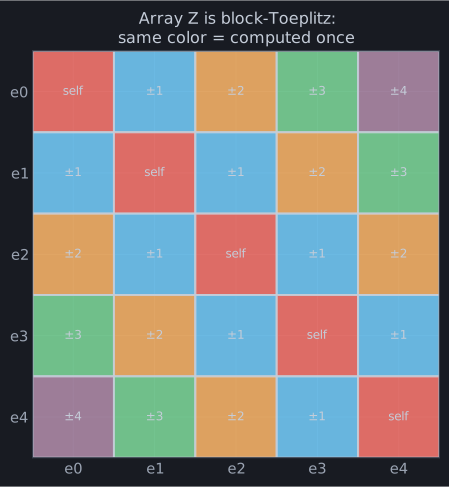
That picture already gives away the two symmetries. First, the self-blocks: identical elements have identical self-interaction, so an element’s block depends only on its shape, not which copy it is. Compute one dense self-block per distinct shape class and reuse it — momwire verified the copies agree to ~2e-12. Second, and stronger, the coupling blocks: in free space the interaction between two elements depends only on their shapes and the displacement between them, never their absolute position. Every block on the same Toeplitz diagonal is therefore the same block. You see it in the figure as the colored stripes — each stripe is computed once.

From P² blocks to a handful

Put the two together — one self-block per shape, one coupling block per unique (shape, shape, displacement) — and the P(P−1) coupling blocks collapse to a short list of keys, each ACA-compressed once (chapter 12) and the reverse direction filled for free by symmetry (Z_ba = Z_ab^T):

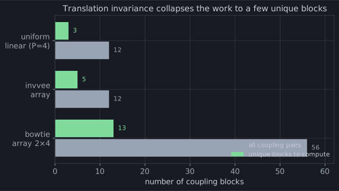
Fifty-six coupling pairs on a bowtie 2×4 become thirteen blocks to actually compute; a uniform line collapses twelve to three. The array’s own regularity did what the H-matrix’s clustering couldn’t see. And the solve is cheap for a third reason: the coupling between elements is weak — about 1e-4 of the self-blocks — so an iterative solve preconditioned by the block-diagonal self-blocks converges in a handful of steps (5 iterations on the inverted-V array, 9 on the bowtie 2×4), landing on the dense BSplineSolver’s impedance to ~1e-5.

This is what lets momwire take a serious multi-element array — the kind where a generic dense solve would be minutes and gigabytes — and answer in the time a few unique blocks take to build. The whole P² grid was only ever a few distinct numbers wearing P² hats.

Toward the epilogue

Step back and look at the machine you’ve assembled across four acts: an integral equation, tamed by a continuous basis; a ground, from a perfect mirror to Sommerfeld’s exact remainder; and a dense matrix, walked through by low rank and symmetry. All of it is Python — readable, the spec you could re-derive. But under the hot loops there is a second copy of the same math, compiled, and a discipline for stopping a solve the instant a knob moves. Chapter 14 lifts that floorboard, and then points you back at the simulator where every bit of this runs live.