10 · Sommerfeld, or paying full price

Chapter 9 left a hole: below about a tenth of a wavelength, the reflection-coefficient mirror is tens of ohms wrong, because the antenna’s near field arriving at the ground is nothing like a plane wave, and a single Γ(angle) can’t describe it. There is no clever weight that fixes this. To get the low antenna right you have to solve the actual electromagnetic boundary-value problem at the air-earth interface — which Arnold Sommerfeld did, for a dipole over a lossy half-space, in 1909.

The exact answer, and its price

Sommerfeld’s solution writes the field as a spectrum of plane waves — an integral over every angle, including the evanescent ones the near field is full of — each reflecting off the interface with its own coefficient. The result is a set of infinite, slowly-converging, oscillatory integrals (the NEC-2 manual writes six of them, on deformed contours that dodge the branch cuts and poles of the ground’s dispersion). It is exact. It is also, done naively, ruinous: every one of the N² source-observation pairs in the matrix would need its own numerical evaluation of those integrals. That’s the “full price” — and paid literally, it puts the exact ground out of reach for anything but a toy.

Don’t integrate what you can subtract

The escape is the idea NEC-2 is built on, and momwire re-derives from the manual’s public equations (_sommerfeld.py, clean-room — no GPL Sommerfeld code consulted). Split the exact field into two parts: an exact image term that carries all the singular, hard-to-integrate behaviour but has a closed form, plus a remainder — everything the perfect image got wrong. Subtract the part you can write down, and what’s left is tame:

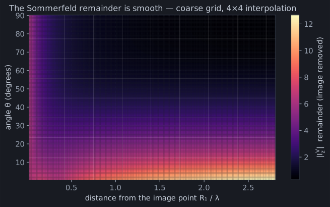
That is the whole trick in one picture. The remainder is smooth — no singularity, no oscillation — a gentle surface over distance and angle. And a smooth surface doesn’t need to be integrated afresh for every pair: compute it once on a coarse grid and interpolate (momwire uses 4×4 Lagrange). The grid depends only on the geometry-independent variables (R₁, θ) and the ground, so a single grid serves all N² interactions in a solve. The impossible per-pair integral becomes a table lookup.

Making exact affordable

That decomposition turns “out of reach” into “costs a grid fill up front”:

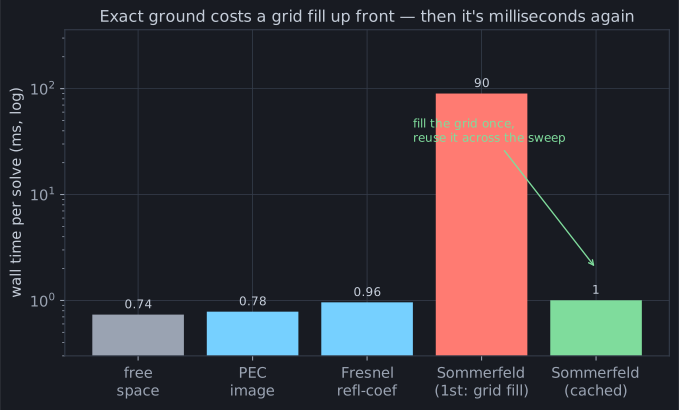
The exact ground’s first solve pays for the grid — here about 100× the cost of the cheap models, and for a big array it’s seconds, not milliseconds. But the grid is cached, so the moment you do anything repetitive — sweep 46 frequencies, drag a height knob in the simulator, refine the mesh — every solve after the first is back to milliseconds. And the grid fill itself has been fought down hard: momwire’s took a documented 12× (4.11 s → 0.34 s for a 2 λ grid) from caching and a fused C++ kernel (docs/sommerfeld-perf-plan.md). That is the difference between a solver you have and a solver you use.

Run it yourself

import numpy as np
from momwire import BSplineSolver

# NVIS dipole a tenth of a wavelength up — where Fresnel was wrong
wire = np.array([[-5.291, 0.0, 0.1 * 22.0], [5.291, 0.0, 0.1 * 22.0]])
solver = BSplineSolver(wires=[wire], nsegs=21, wavelength=22.0, wire_radius=0.0005,
                       degree=2, ground_z=0.0, ground_eps=(13.0, 0.005),
                       ground_model="sommerfeld",       # <- pay full price, get it right
                       feed_wire_index=0, feed_arclength=5.291)
Z, _ = solver.compute_impedance()
print(f"Z_in = {Z.real:.0f} {Z.imag:+.0f}j ohms")   # ~53 -6j — vs Fresnel's 47 -3j

Act III, closed

You climbed the ground ladder rung by rung:

• PEC (ch. 8): one extra kernel term, a perfect mirror, free — and the height oscillation every operator has felt;
• Fresnel (ch. 9): the mirror dimmed by a reflection coefficient, exact above ~0.15 λ for almost the same price;
• Sommerfeld (ch. 10): the real boundary-value problem, exact everywhere, made affordable by subtracting the image and interpolating the smooth remainder.

Everything so far has been about getting the physics right. Act IV is about getting it fast enough to matter — because a dense N×N matrix is a wall, and the whole business of momwire, from H-matrices to array symmetry to the compiled kernels, is the story of walking through it.