3 · The feed and the answer
Chapter 2 ended owing two explanations: the feed line we typed without comment, and the question of how many segments the toy’s “working” answer actually cost. Start with the feed, because it is the antenna’s connection to the outside world.
What “1 volt in a gap” became
Section titled “What “1 volt in a gap” became”In the toy, the generator turned into exactly one line:
v[N // 2] = 1.0That is the delta-gap source: pretend the generator’s 1 volt appears entirely across the feed segment, producing an applied field there and nothing anywhere else. It’s the crudest workable model of a feed — no coax, no balun, just a voltage jump — and it is what virtually every wire code uses by default.
momwire’s delta-gap is the same move. Inside
compute_impedance,
the right-hand side is built as
v[fi] += -V_i / geom["seg_h"][fi]
— voltage over feed-segment length, with the sign and constants absorbed into
the solver’s conventions. Same idea, a better-tested version of it — though,
as we’re about to see, the feed is not where the toy’s last ohm hides.
Solve the system, read off the current where the generator sits, and the number every ham actually wants falls out:
Z_in = V / I(feed) = 1 / I[N // 2]Drive-point impedance. SWR is a one-line formula away from it; “resonance” means its imaginary part crosses zero. When this chapter ends, we’ll sweep it across frequency and watch that happen.
How many segments did that cost?
Section titled “How many segments did that cost?”Chapter 2 quoted the toy at N = 161: 70.9 − 8.7j, against momwire’s settled
69.6 − 18.3j. Close on the resistance, loose on the reactance. The honest
question is what happens as we refine — and the answer is the most instructive
picture in naive MoM:
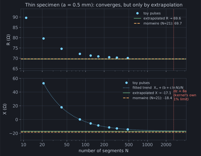
It converges — no window, no collapse, just a steady approach to the right answer. But look how unevenly:
- The resistance settles fast. By a couple hundred segments
Ris within an ohm, and its error is clean first-order (∝ 1/N). Three coarse solves and a Richardson extrapolation land it dead on69.6. - The reactance crawls. At
N = 481— half a thousand unknowns —Xis still only−14.4, several ohms shy. And it doesn’t ride a clean1/N: the self-termlog(dz/a)from chapter 2 injects a logarithm, so the reactance followsX ≈ X∞ + (b + c·log N)/N. Fit that curve (the dotted line) and you can extrapolate toX∞ ≈ −17from coarse data — a real rescue, pulling a usable estimate out of solves that individually look nowhere near it. (Don’t read too much precision into it: the fit pinsX∞to a couple tenths, not a hundredth.)
So: yes, you can get final values out of the pulse method. But count the cost.
The resistance needs a handful of solves and a one-line extrapolation. The
reactance needs many solves, a fitted model of its trend, and even then lands
about an ohm short of a good basis — because the last ohm isn’t a
convergence error at all. Notice R extrapolates exactly onto momwire while
X stops an ohm away: an offset in the reactance alone, untouched by refining,
is the fingerprint of the basis — not a convergence error, and (perhaps
surprisingly) not the feed. The pulse’s staircase resolves the near-field
reactive energy that X is made of a little differently than a continuous
basis does, and settles about an ohm off; smoothing the delta-gap into a
finite-width source — or a coaxial “frill” — barely moves it. Only a better
basis closes that gap, which is what Act II is.
And brute force is no escape hatch. To reach the converged reactance without
extrapolating, you’d shrink the segments until dz approached the wire radius
— but the thin-wire kernel has its own limit, roughly dz > 8a for 1% accuracy
(the red line, thousands of segments out). Push past it and the kernel itself
is wrong; you’d be converging a coarse approximation to the wrong number. The
pulse method makes you choose between a curve fit and a fortune in unknowns,
and hands you an approximate feed either way.
Why so slow — and the thread into Act II
Section titled “Why so slow — and the thread into Act II”Why does the reactance, of all things, crawl the worst? The clue is where we
put the charge. X is near-field, reactive energy — and near-field energy is
mostly the scalar potential, the field of those charge piles at the segment
endpoints. A pulse current is discontinuous, so its charge lands in
concentrated knots at the joints; the potential of a knot is a crude,
slowly-improving thing, and it dominates the reactance. Resolving it is exactly
what the extra segments are struggling to do.
That single observation is the hinge of the whole primer. Make the current
continuous and its charge stops piling into knots and spreads into honest,
distributed charge — the scalar potential converges, the reactance snaps into
place, and you need a handful of segments instead of hundreds. Every basis
momwire ships is continuous, and Act II is the story of what that buys:
SinusoidalSolver and BSplineSolver nail this same dipole — resistance and
reactance — at twenty-one unknowns, no extrapolation, in milliseconds. You
cannot cheaply out-refine a staircase; you can only stop drawing one.
The payoff plot
Section titled “The payoff plot”One number is an appetizer. The answer a ham actually plots is the impedance
across the band — and now that solves in one call. The swept solver
(compute_impedance_swept)
takes an array of wavenumbers:
import numpy as npfrom momwire import SinusoidalSolver
wire = np.array([[0.0, -5.291, 0.0], [0.0, 5.291, 0.0]])solver = SinusoidalSolver(    wires=[wire],    nsegs=81,    wavelength=22.0,    wire_radius=0.0005,    feed_wire_index=0,    feed_arclength=5.291,)  # 1 V gap at the centerlams = np.linspace(18.0, 27.0, 46)  # 46 frequenciesZ = np.asarray(solver.compute_impedance_swept(2 * np.pi / lams)).ravel()
46 frequencies in 65 ms, and the classic textbook curve appears — generated by your specimen, not copied from a book:
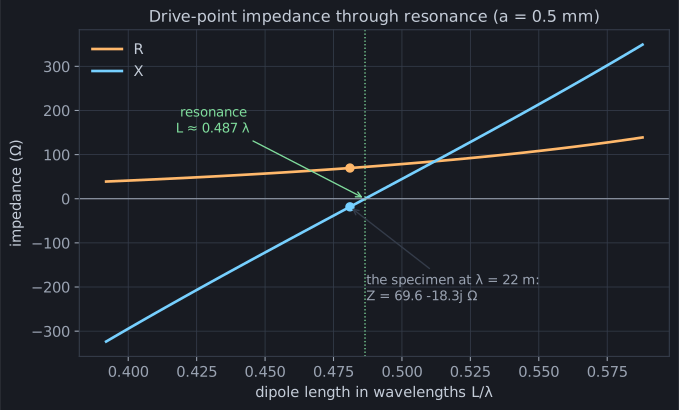
Everything a ham knows by feel is in that picture, computed from first
principles: the dipole is capacitive when short, inductive when long, and
resonates (X = 0) at L ≈ 0.487 λ — a hair under a half wave, exactly the
“cut it a few percent short” rule of thumb, which for this wire is the
thickness correction made visible. Our specimen sits just below resonance at
λ = 22 m, which is why its reactance is −18 Ω.
Act I, closed
Section titled “Act I, closed”You now own the core of the method of moments, honestly:
- an antenna question is an integral equation for the current (ch. 1),
- a basis + testing scheme turns it into
Z·I = V, and even the crudest choice — pulses on the 2n+1-point grid — works (ch. 2), - the feed model supplies
V, andZ_in = V/I(feed)is the answer (ch. 3), - but the naive basis converges slowly and unevenly, buying its final digits only with extrapolation or a flood of unknowns — which is why the craft of Act II, better bases, is not a luxury.
Act II opens inside that craft: what makes NEC’s strange little
constant + sine + cosine basis so unreasonably effective that twenty-one
unknowns nail a dipole to a tenth of an ohm — reactance and all.