4 · Sinusoids, NEC's bet

Act I closed on a promise: the pulse toy crawled because a discontinuous current dumps its charge into concentrated knots at the segment joints, and the scalar potential of those knots — where the reactance lives — converges only first-order. Make the current continuous and the knots spread into honest distributed charge. This chapter cashes that promise, with the basis NEC-2 has used since 1981.

The bet

Look again at what the current on a wire actually does. Chapter 1 turned the antenna into an integral equation; strip it to its skeleton and the current obeys, near enough, (d²/ds² + k²) I ≈ source — the wave equation along the wire. And the solutions of (d²/ds² + k²)·f = 0 are exactly sin ks and cos ks. The current wants to be a sinusoid; it only bends away from one where the wire ends, kinks, or is fed.

So make that the bet. On each segment, expand the current in the three shapes a sinusoid can locally be:

I_j(s) = A_j + B_j·sin k(s − s_j) + C_j·cos k(s − s_j),   |s − s_j| < Δ_j/2

A constant, a sine, a cosine — NEC-2’s three-term basis (Burke & Poggio 1981, Eq. 20; the momwire re-derivation is in docs/sinusoidal_basis_design.md). The coefficients aren’t free: across each joint the basis enforces continuous current and continuous slope, with Kirchhoff’s current law baked into the shapes at junctions — so there is still exactly one unknown amplitude per segment, an N×N matrix, same size as the pulse toy. Here are three of these basis functions, pulled straight out of SinusoidalSolver:

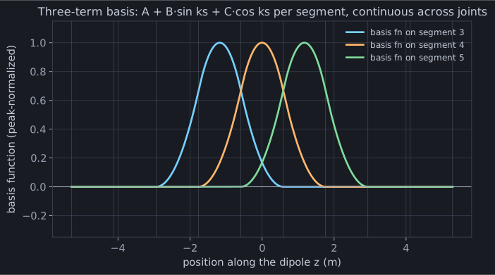
Set that beside chapter 2’s staircase of boxes. Those were discontinuous — a cliff at every joint, a charge knot behind each cliff. These are smooth, they overlap, and they meet their neighbours with matching value and slope. That single change — continuity — is the entire difference between crawling and converging.

Five segments

How much does it buy? Give the specimen dipole five segments and read the current off both bases:

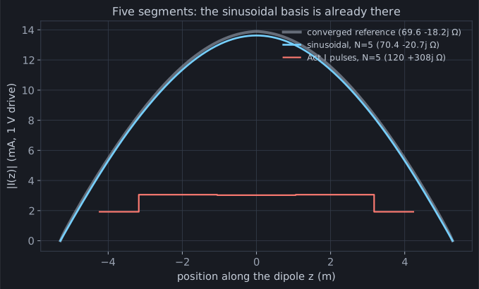
The sinusoidal current, with five unknowns, is already lying on the converged answer — 70.4 − 20.7j against the true 69.6 − 18.3j. The Act I pulse toy at the same five segments returns 120 + 308j and a current that isn’t remotely the right shape. Refine a little and the sinusoid locks on:

N	sinusoidal	Act I pulses
5	70.4 − 20.7j	120 + 308j
7	70.0 − 19.8j	103 + 207j
21	69.7 − 18.7j	80 + 53j
81	69.63 − 18.30j	72 − 1j

Twenty-one sinusoidal unknowns beat five hundred pulses — reactance and all, the thing the pulse could never buy at any price. The continuous current has an honest, distributed charge, so the scalar potential that carries the reactance converges as fast as everything else.

The wave equation does the integral

There’s a second gift, and it’s the one that makes this basis cheap, not just accurate. Filling the matrix means computing the field each basis shape radiates onto every segment — an integral of the current against chapter 1’s kernel. For a general current that integral is real work (chapter 6 is entirely about it). But watch what the wave operator does to a sine:

(d²/ds² + k²) · sin ks = 0

The field of a wire current runs through exactly that operator — and it annihilates sin ks and cos ks. So the field of a sine-current segment, and of a cosine-current segment, collapses to a closed-form expression evaluated at the two segment endpoints — no integral at all (Burke & Poggio Eqs. 76–79). Only the constant component still carries an honest integral (k² ∫ G₀ ds'). Two of the three basis shapes fill themselves for free, because the basis was chosen to be what the physics already solves. That is NEC’s bet paying its second dividend: pick the basis the operator likes, and the operator does most of your quadrature.

The sharpest ruler

There’s a reason momwire carries this basis at all, given it also ships smoother, more general ones (chapter 5). Because it is NEC-2’s exact basis — same three terms, same testing, same thin-wire kernel — it is momwire’s sharpest cross-validator. On the specimen dipole, momwire’s sinusoidal solver returns 69.63 − 18.30j; NEC-2 (via PyNEC), on the identical geometry, returns 69.64 − j18.21 (docs/convergence_analysis.md). A tenth of an ohm apart — two independently written codes, agreeing to the fourth significant figure. When two solvers share a basis and disagree, the disagreement has to live in the kernel, the feed, or the junctions; matching NEC here is what lets momwire isolate and trust every other piece. Chapter 7 makes that cross-validation the credibility anchor of the whole engine.

Run it yourself

import numpy as np
from momwire import SinusoidalSolver

wire = np.array([[0.0, -5.291, 0.0], [0.0, 5.291, 0.0]])
solver = SinusoidalSolver(wires=[wire], nsegs=5, wavelength=22.0,
                          wire_radius=0.0005,
                          feed_wire_index=0, feed_arclength=5.291)  # 1 V at the center
Z, alpha = solver.compute_impedance()
print(f"N=5:  Z_in = {Z.real:.1f} {Z.imag:+.1f}j ohms")   # 70.4 -20.7j — five segments!

If the sinusoidal basis is this good on a straight dipole, why does momwire lean on B-splines for real antennas? Because a real antenna bends, branches, and meets itself at junctions — and NEC’s gorgeous closed-form coefficients turn hairy the moment the wire stops being straight. Chapter 5 trades a little of this magic for a basis that stays simple on any shape.

Turn the knob yourself

The antennaknobs simulator runs this engine live — drag a dipole’s length and watch Z_in track resonance in real time.