8 · Mirror worlds

Everything in Acts I and II floated in free space. Real antennas don’t: they hang over the earth, and the ground rewrites their impedance and their pattern. Act III adds it back, one layer of realism at a time. Start with the simplest possible ground — a perfect conductor — because it costs almost nothing and it already reproduces the effect every operator knows by feel.

The oldest trick

A perfect electric conductor forces the tangential electric field to vanish on its surface. You could enforce that with a wall of unknowns across the whole plane — or you could use the trick Lord Kelvin published in 1848. Replace the ground with a mirror image of the antenna, the same distance below the plane, carrying a current arranged so the two together satisfy E_tan = 0 automatically. For a horizontal wire, the image current runs backwards:

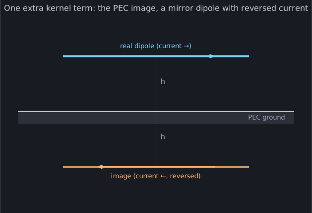
Above the plane, the field of {antenna + image} is identical to the field of {antenna + real ground} — and now there’s no ground to mesh, just a second wire that isn’t even an unknown. Its current is dictated, point for point, by the real antenna’s. In the method of moments this is almost insultingly cheap: every matrix entry gains one extra kernel term — the field of segment n’s image evaluated at segment m — and nothing else changes. Same unknowns, same matrix size. In momwire it’s a single constructor argument, ground_z: set the plane’s height and the solver reflects every segment for you.

Height is a knob

Once the image is in, the antenna feels its own reflection — and the feel depends entirely on how far above the ground it sits, because the round trip down to the image and back is a path length that slides in and out of phase:

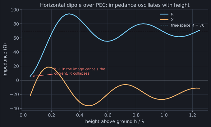
Read it from the left. At very low height the image is right underneath, its reversed current almost perfectly cancelling the real one — the radiation resistance collapses toward zero. A horizontal dipole lying on a perfect ground is a short circuit; it can’t radiate, because its mirror twin is fighting it at point-blank range. Lift it to about 0.3 λ and the reflection comes back in phase — R peaks near 94 Ω, well above free space. Keep going and the impedance oscillates, each swing smaller than the last, converging on the free-space 69.7 Ω as the ground recedes out of reach.

That oscillation is not a numerical artifact; it is the single most practical fact about antenna height. Every operator who has raised a dipole and watched the SWR change has measured this curve. It’s why “get it up at least a half-wavelength” is folklore, and why a low antenna feeds so strangely.

Run it yourself

import numpy as np
from momwire import BSplineSolver

# horizontal half-wave dipole, 0.3 lambda up, over perfect ground at z = 0
h = 0.3 * 22.0
wire = np.array([[-5.291, 0.0, h], [5.291, 0.0, h]])
solver = BSplineSolver(wires=[wire], nsegs=21, wavelength=22.0, wire_radius=0.0005,
                       degree=2, ground_z=0.0,          # <- the whole ground model
                       feed_wire_index=0, feed_arclength=5.291)
Z, _ = solver.compute_impedance()
print(f"Z_in = {Z.real:.0f} {Z.imag:+.0f}j ohms")   # ~93 +5j — up from 70 in free space

One argument, one extra kernel term, and the dipole knows there’s a floor. But the earth is not a perfect conductor — it’s dirt, imperfectly reflecting and quietly absorbing. The mirror is real but dim, and its dimness is complex and angle-dependent. Chapter 9 replaces the perfect image with the next honest approximation: the Fresnel reflection coefficient.