6 · Integrals done honestly

The sinusoid of chapter 4 filled two-thirds of its matrix for free, because the wave operator annihilated its sine and cosine pieces. The B-spline of chapter 5 has no such luck: a polynomial current is not a solution of the wave equation, so every matrix entry is a genuine integral of chapter 1’s kernel against two basis functions. Most are easy. A few will ruin your day. Telling them apart — and treating each honestly — is the unglamorous craft that decides whether the whole solver is accurate. As the saying in this field goes: MoM is 90% quadrature engineering.

Two neighbours, two integrands

Filling entry Z[m][n] means integrating the kernel g(s, s′) = e^{−jkR}/(4πR) as the source point s′ runs across segment n and the observation point sits on segment m. Whether that integral is trivial or treacherous depends entirely on how far apart the two segments are:

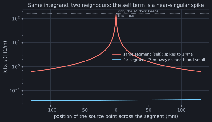
For a far pair, the integrand is a gently curved line — the kernel barely changes as the source crawls across a distant segment. For the self pair (and its close neighbours), the source point passes directly under the observation point, R collapses toward the wire radius a, and the integrand spikes to 1/4πa — here about 160, held finite only by chapter 1’s a² floor. Same formula, wildly different shape, and Gauss-Legendre quadrature feels the difference brutally.

You can’t out-integrate a singularity

Point a fixed quadrature rule at both and watch:

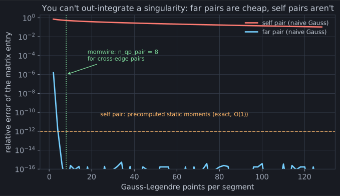
The far pair is nailed to machine precision by four points — the integrand is smooth, and Gauss quadrature is exact for smooth things almost immediately. The self pair is a disaster: at one hundred and thirty points it is still ~100% wrong. The spike is half a millimetre wide sitting in a segment a quarter of a metre long; the Gauss nodes step right over it, never seeing the thing that carries most of the integral. Adding points barely helps — you would need nodes spaced finer than a across the whole segment, thousands of them, and even then you’d converge slowly. This is the same wall Act I’s pulse toy hit, and the same lesson: you cannot out-integrate a singularity; you have to handle it.

The split

So momwire refuses to try. It splits the two cases and gives each what it needs (BSplineSolver, constructor knobs n_qp_pair and the static-moment path):

• Far and near-but-not-touching pairs get plain Gauss-Legendre — from the memoized _quadrature.py (all thirty lines of it: leggauss is not free, so cache it). Since momwire#743 the order is two knobs rather than one, because the two cases want different things: n_qp_pair = 8 for cross-edge pairs (two different edges), and n_qp_pair_same_edge = 4 for the smooth remainder of a same-edge pair. Four is plenty for the far pair plotted above; it is not plenty for two edges that nearly touch, and that margin is what the cross-edge default buys.
• Self and edge-sharing pairs get the singular integral precomputed analytically as static moments — the integral of the 1/R singularity against each pair of B-spline pieces, worked out once in closed form (scripts/derive_bspline_static_moments.py → the big table in _bspline_static_moments.py). At runtime the treacherous entry is a table lookup, not an integral.

They’re called static moments for a reason worth its own sentence: the singular geometry — how a 1/R behaves against two overlapping splines — does not depend on frequency. So it’s computed once and reused at every wavenumber. When chapter 3’s swept solver evaluated 46 frequencies in 65 ms, this is why: the hard part of every matrix was already done, frequency-free.

Run it yourself

On a straight dipole this scheme has nothing left to prove. Since the knob was split, n_qp_pair there is not merely converged but inert — one edge means no cross-edge pairs at all:

import numpy as np
from momwire import BSplineSolver

wire = np.array([[0.0, -5.291, 0.0], [0.0, 5.291, 0.0]])
for nq in (2, 4, 8):
    Z, _ = BSplineSolver(
        wires=[wire],
        nsegs=21,
        wavelength=22.0,
        wire_radius=0.0005,
        degree=2,
        n_qp_pair=nq,
        feed_wire_index=0,
        feed_arclength=5.291,
    ).compute_impedance()
    print(f"n_qp_pair={nq}:  {Z.real:.4f} {Z.imag:+.4f}j")
# n_qp_pair=2:  69.6635 -18.3652j
# n_qp_pair=4:  69.6635 -18.3652j
# n_qp_pair=8:  69.6635 -18.3652j   — bit-identical: no cross-edge pairs to integrate

The knob that does move on this deck is the other one, and it moves by two-thousandths of an ohm across the whole range — swap n_qp_pair=nq for n_qp_pair_same_edge=nq above:

# n_qp_pair_same_edge=2:  69.6634 -18.3665j
# n_qp_pair_same_edge=4:  69.6635 -18.3652j
# n_qp_pair_same_edge=8:  69.6635 -18.3648j

Where it is not inert

A dipole is the easy case, and for a long time it was the only case anyone measured. On a crossing junction at a lossy-soil interface the cross-edge integrand is near-singular rather than smooth, and the error falls only as C/q with C ≈ 33 — first order in the number of Gauss points, which is a lost convergence rate, not a slow one (momwire#760). On the soil-A crossing fan:

n_qp_pair	Z	distance from the limit
4	142.1923 − 36.4707j	6.808 Ω
8	141.3991 − 40.6483j	2.556 Ω
16	141.0601 − 42.4754j	0.698 Ω
64	140.9366 − 43.1577j	0.005 Ω

That class is why the cross-edge default moved from 4 to 8, and why buried decks resolve to 32. The accelerated kernel’s n_qp² ≤ 64 scratch buffer used to bind here — reaching the bottom row needed the numpy path — until momwire#762 made the buffer a tile width, so every order in that table now runs accelerated. The honest summary is narrower than this chapter used to claim: the smooth-pair quadrature is as settled as the dipole makes it look for smooth pairs, and a near-singular cross-edge pair is not one.

Paying the high order only where it is owed

A radial screen of 654 buried segments has 428,000 segment pairs, and at order 32 each one paid a 1,024-point grid — two calls of one kernel were 6.3 of the solve’s 11.3 s. But the near-singular class above lives on the pairs that nearly touch; a pair sixteen segment lengths apart is the far pair of the figure at the top of this chapter, at machine precision by 4 points. Binning every pair’s error by its centre distance over the longer segment made that exact (momwire#906): order 8 is within 1e-13 of order 32 beyond two lengths, order 4 within 3e-14 beyond sixteen, for real and lossy-medium wavenumbers alike, and the order-8 threshold does not care about electrical length at all (the order-4 tier does, so a block whose longest segment passes kL = 0.5 loses it).

So the cross-edge order is now a ladder: buried decks run 32 on the pairs under two lengths apart — about one pair in a hundred on that screen — 8 out to sixteen lengths, and 4 beyond, which is 87 % of them. The two kernel calls went from 2.4 s each to 0.08 s at the same impedance to every printed digit, and the 12-radial screen from 11.3 s to 5.7 s. Free space keeps a single order for now, until the same flip is measured there (momwire#907).

The matrix is now filled honestly — smooth where it can be, exact where it must be, and explicit about the one place the smooth rule strains. Which raises the question this whole act has been circling: filled honestly or not, how would you know the final answer is right? Chapter 7 is the cross-examination — convergence, the knee, and an independent engine.