1 · The question

Here is the entire subject of this site, in one picture:

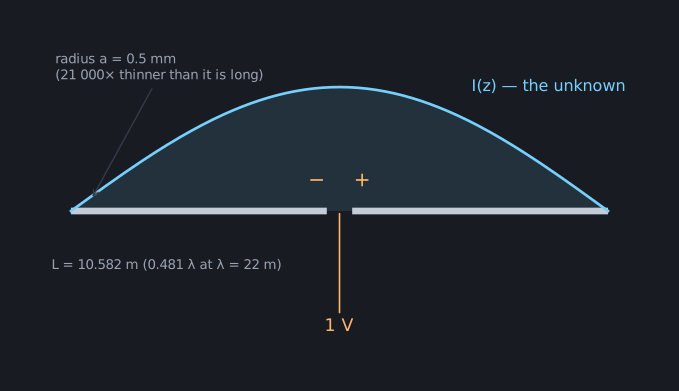
A straight wire, 10.582 m long and half a millimetre in radius, cut in the middle. A generator drives 1 volt across the cut. The question: what current I(z) flows along the wire?

That’s it. Everything an antenna tool tells you is downstream of this one unknown. The drive-point impedance — the number your SWR meter argues with — is just 1 V / I(feed). The radiation pattern is a weighted sum of the current at every point. Gain, resonance, coupling to a neighbouring element: all functionals of I(z). Answer the question and you’ve answered everything.

This wire is the specimen for the whole primer. It’s momwire’s own default antenna — a dipole of length 0.481 λ at λ = 22 m (13.6 MHz), which those constructor defaults wavelength=22, halfdriver_factor=0.962 describe — and it will follow us through every chapter, getting solved by progressively better machinery.

Why this is hard

You might hope for a formula. There isn’t one — and it’s worth seeing exactly why, because the shape of the difficulty dictates the shape of every solver in this field.

A current element at position z′ produces an electric field everywhere in space, including at every other point z on the wire. Meanwhile the wire is (nearly) a perfect conductor, which imposes a hard rule: the total tangential electric field on its surface must be zero — everywhere except inside the gap, where the generator applies its field.

Put those two facts together. The field at z produced by the whole current distribution is a sum — an integral — over contributions from every z′:

E_scattered(z) = ∫ I(z′) · K(z, z′) dz′

where K(z, z′) (the kernel) encodes “how much field a unit of current at z′ produces at z”. The boundary condition then says:

∫ I(z′) · K(z, z′) dz′ = −E_applied(z)     for every z on the wire

This is Pocklington’s integral equation. Notice what kind of beast it is: the unknown I(z′) lives inside the integral. It isn’t one equation — it’s a continuum of them, one for every observation point z, all coupled to the current everywhere else. The current at the feed depends on the current at the tips, which depends on the current at the feed. You cannot march along the wire computing it locally; the whole distribution must be found at once.

Hold onto that word “coupled” — it’s why, three chapters from now, we’ll be staring at a dense matrix, and why in Act IV the cost of that matrix becomes the villain of the story.

Where’s Maxwell?

One step upstream. K(z, z′) is built from the free-space Green’s function e^(−jkR)/4πR — the field of a point source oscillating at frequency k = 2π/λ — pushed through the derivatives that turn a vector potential into an electric field. This primer treats the kernel as a given physical ingredient and spends its energy on what solvers do with it. The NEC-2 theory manual derives it in full if you want the provenance.

The thin-wire trick

There’s a mathematical landmine in that integral. The kernel contains 1/R-type terms, where R is the distance between source and observation point. When z → z′ — the field of a piece of wire at itself — R → 0 and the kernel blows up.

The classical escape uses the wire’s one merciful property: it’s thin (our specimen is 21 000× thinner than it is long). So:

1. Pretend the current flows along the wire’s axis.
2. Enforce the boundary condition on the wire’s surface, one radius away.

Source and observation point now live on different lines, and the distance becomes

R = √( (z − z′)² + a² )

which can never fall below the wire radius a. The singularity is gone — replaced by a sharp but finite peak:

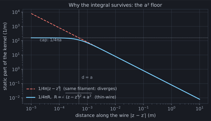
This a² under the square root is the signature of every thin-wire MoM code on earth, and you can watch momwire apply it verbatim: the sinusoidal solver’s field evaluation computes rho_eval = np.sqrt(rho_axis * rho_axis + a * a) — the perpendicular distance floored at one radius — and the B-spline solver’s module header declares “thin-wire kernel with a² wire-radius regularization” as a design commitment in its first lines.

Nothing is free: the peak is still violently sharp. For our specimen the kernel varies on a length scale of half a millimetre near the diagonal, on a wire ten metres long. Integrating across that peak accurately is where an enormous amount of solver craft goes — Act II devotes a whole chapter to it, and the toy solver we build in the next chapter will be wrecked by it in an instructive way.

What “solving” means now

So the problem statement is fixed: find the function I(z) that makes the scattered field cancel the applied field along the entire wire. An unknown function, pinned down by an integral equation.

Computers don’t solve for functions. They solve for finitely many numbers. The whole method of moments is the art of turning this integral equation into a finite matrix equation honestly — and that’s the next chapter.

Run it yourself

The machinery of the next two chapters, applied to this exact specimen (momwire is on PyPI: pip install momwire):

import numpy as np
from momwire import SinusoidalSolver

wire = np.array([[0.0, -5.291, 0.0], [0.0, 5.291, 0.0]])  # the specimen, 10.582 m tip to tip
solver = SinusoidalSolver(wires=[wire], nsegs=81, wavelength=22.0,
                          wire_radius=0.0005,
                          feed_wire_index=0, feed_arclength=5.291)  # 1 V gap at the center
Z, currents = solver.compute_impedance()
print(f"Z_in = {Z.real:.1f} {Z.imag:+.1f}j ohms")   # Z_in = 69.6 -18.3j ohms

That feed_arclength=5.291 — half the wire’s length — is the delta-gap feed sitting at the electrical center; it’s also the default, but a feed is a choice (move it and you have an off-center-fed antenna), so we name it. 69.6 − 18.3j Ω, in about 2 ms. By the end of Act I you’ll know exactly what had to happen inside that call — and you’ll have built the obvious naive version yourself and watched it work, just slowly enough to see why momwire doesn’t stop there.

Turn the knob yourself

The same engine runs live in the antennaknobs simulator — drag a dipole’s length knob and watch Z_in move in real time.